
I admit “Basic” and “Machine Learning” are two phrases that do not belong together in the same sentence. However, with much of today’s attention focused on generative artificial intelligence (GAI) systems like Large Language Models (LLMs), it is easy to overlook the value of foundational machine learning in solving practical, data-intensive problems. Indeed, machine learning remains a cornerstone of predictive analysis, optimization, and decision-making across industries. For example, in my own work, I have applied machine learning algorithms to stock trading, semiconductor manufacturing decision systems, and most recently, to the challenge of forecasting energy demand. This article explores the value of foundational machine learning approaches, how to expand on these techniques, and how to apply practices to real world problems. It focuses on forecasting energy demand and summarizes my experience building a feed-forward neural network with backpropagation from scratch.
From Dollars to Megawatts: Building Trust in Machine Learning Models
I recently completed the course Machine Learning for Trading as part of my Master’s program. As part of the course, I implemented a regression tree from scratch, extended it into a classifier, and later developed a Q-Learner. For the final project, the models were trained on historical data from JPMorgan Chase & Co ($JPM) covering 2008-2009 and evaluated from 2010-2011. The trading algorithm was able to enter a long, short, or neutral position, with trades executed at the start of each day based on signals from the previous trading session.
In addition, the algorithm was provided with a number of other metrics including price momentum, moving average convergence divergence (MACD), flattened bollinger bands, relative strength index (RSI), and a flattened golden cross signal. These signals use the same price data to be calculated but provide additional contextual information to the decision tree. This process of creating “new” data from existing data is often known as feature engineering or feature extraction.
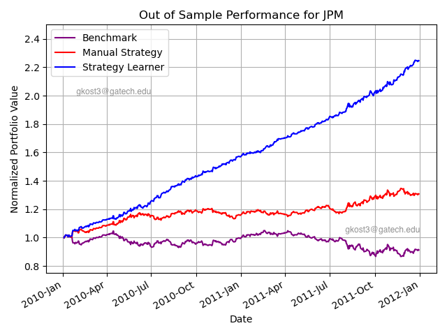
Figure 1: Results of classifier learner compared to manual tuning and benchmark portfolio.
As seen in Figure 1 above, the strategy learner (in this case, a regression classifier) achieved remarkable results with over a 220% return, far outperforming the buy-and-hold benchmark and manually tuned trading strategies. In fact, these results were so good, they initially seemed too good to be true, but my peers were reporting similar results.
How could a student develop such an effective strategy outperforming the top hedge funds in just a single semester on normal consumer-grade hardware? I questioned the choice of $JPM and the date range used for the class standard—maybe the professor chose this particular dataset for a reason. Perhaps, a simple classifier strategy learner would be less effective today with the explosion of algorithmic trading and AI/ML advancements. Repetitive excess gains (alpha) are generated through a competitive advantage. However, when the classifier was retrained on data for 2023-2024 and tested January 2024 to October 2025, similar results were seen across industries.Figure 2 shows, out of sample performance for $JPM, $XOM, $BA, and $NVDA with remarkable results.
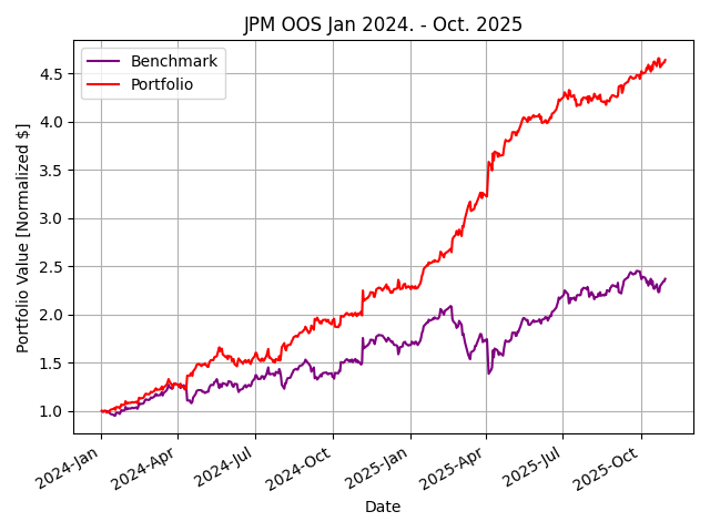
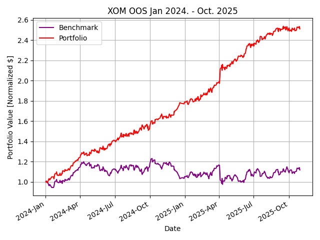
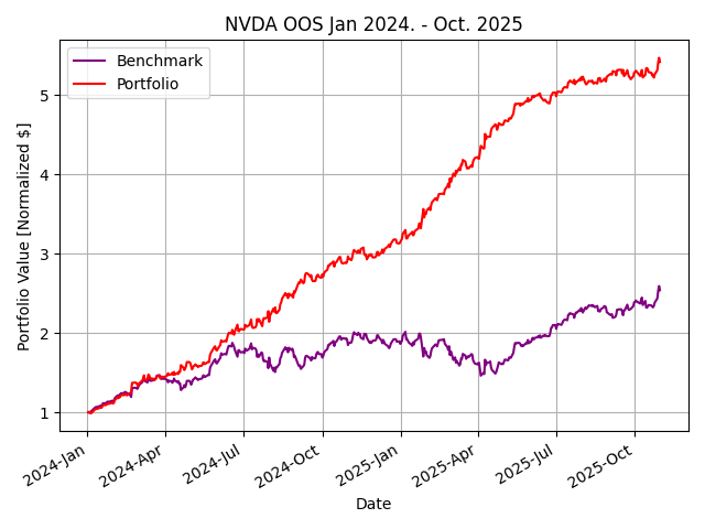
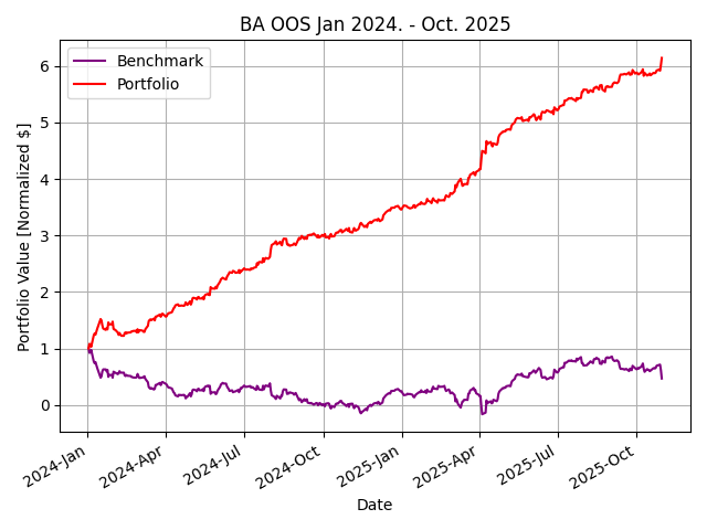
Figure 2: Results of classifier learner out of sample from January 2024 to October 2025
The extraordinary returns are likely a result of extreme simplifications used by the class to highlight the workings of machine learning algorithms. While brokerage commission and market slippage (price changes due to large orders) are considered, bid-ask spread, and other sources of inefficiencies degrade the returns in real-world markets. In addition, the strategy of 100% long or 100% short used in the class results in small returns compounding extremely quickly.
Finally, the largest limitation of this strategy is that it assumes infinite liquidity, the ability to short at any time, no margin requirements, a magical order execution (i.e. no partial order fills), all of which are impossible to find in real markets. Under these conditions, even small predictive edges compound, resulting in returns that are not possible in real markets. By contrast, top-performing quantitative hedge funds return 20-30% annually over multi year periods when considering these details.
In spite of these limitations, machine learning algorithms can be effective for time-series forecasting and can be applied to applications such as trade decisions through thoughtful data engineering techniques. There are a number of applications where time-series forecasting does not have the same constraints as capital markets, such as energy demand forecasting, predictive maintenance from IoT sensor data, medical monitoring, and process controls.
Building a Neural Network
Given the success of my earlier work, I wanted to try applying these techniques to a new problem: forecasting energy demand. I followed a great tutorial from Andres Berejnoi on implementing backpropagation in a neural network built from scratch.
For data, I used the U.S. Energy Information Administration’s Electricity Balancing Authority (EBA) dataset. Specifically, I selected a single interconnection between PacifiCorp West (PACW) and Bonneville Power Administration (BPAT) to keep the dataset relatively small for this proof of concept. With this dataset, it was feasible to predict the next hour’s energy exchange value with the provided historical observations.
However, simple feed-forward neural networks lack temporal memory, a significant limitation when attempting to forecast time-series data. Essentially, each input sample is treated independently, with no inherent mechanism for learning how past values influence future ones. As a result, when trends or cyclical patterns span hours or days, the model quickly loses context. As you might expect, electricity demand is highly cyclical, presenting a significant challenge to applying the scratch-built neural network to this specific problem.
To understand this challenge from a more technical side, the neuron in a simple feed-forward network performs a single calculation. This calculation is directly dependent on the inputs and does not maintain any state, therefore cyclical patterns are lost to the model. You can think of this neuron as a worker with no memory: it only sees the current hour’s demand and makes a decision based on the sole data point, forgetting what it observed in previous hours.
However, a modification of the simple neuron adds statefulness to it. In the worker analogy, this worker (neuron) now has a notebook where it can record previous observations to strengthen its predictive power. With this enhancement, the neuron (worker) performs three operations: what to forget (scratches out old observations from the notebook) , what to remember (writes down new observations), and what to output (what decision to make). This modification is the foundation of Long Short Term Memory (LSTM) networks, a stateful neural network that remembers relationships across time. For now, I have elected to make use of TensorFlow’s LSTM module.
The Challenges: Gradient Explosion and Instability
Building a neural network with TensorFlow is programmatically simple, though there are some underlying configurations a developer needs to make knowledgeable decisions about, such as network size, activation function, use of an optimizer, epochs, and batch size.
# create network topology with 50 neurons and a single output neuron that is
# connected to every neuron in the preceeding layer (densely connected)
num_neurons = 50
model = Sequential([
  LSTM(num_neurons, activation='tanh', input_shape=(n_steps, 1)),
  Dense(1)
])

# Use an optimizer with gradient clipping
optimizer = tf.keras.optimizers.Adam(clipnorm=1.0)

# Compile network
model.compile(optimizer=optimizer, loss='mse', metrics=['mae'])

# train the model
history = model.fit(
  X_train, y_train,
  epochs=15, # number of iterations through entire data set
  batch_size=32, # number of samples before each weight update
  validation_split=0.2,# use 20% of data to validate, 80% to train
  verbose=1 # print out progress of each epoch
)
Initially, my configuration resulted in NaN values during training for loss and mean absolute error (MAE). After debugging and research, it appears that this issue is indicative of gradient explosion, a quirk where neuron weights exponentially grow to unmanageably large values.
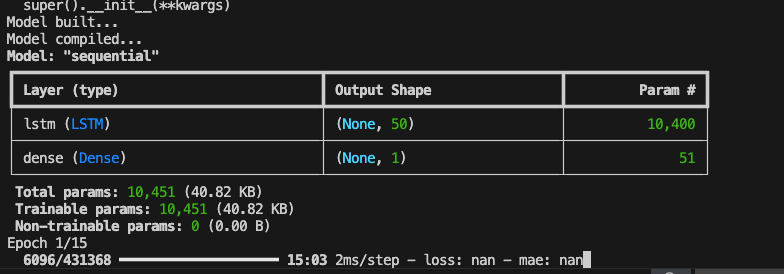
Figure 3: Verbose terminal output from TensorFlow showing “nan” values for initial training with 15 epochs and 50 neurons. NaN values are indicative of gradient explosion issues.
To stabilize the model, I first scaled my data and ensured any NaN values were dropped from the data set. Further, I switched from the ReLU to tanh activation functions. Tanh squashes inputs between -1 and 1, while ReLU does not have an upper bound on values.
I also added the optimizer (seen above) to increase convergence speed. Optimizers are algorithms that adapt to the magnitude of weight changes allowing the model to learn faster and more efficiently. The Adam optimizer was chosen because it utilizes adaptive learning rates with value momentum, making it particularly well suited for time-series forecasting.
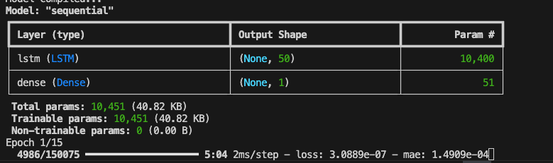
Figure 4: After corrections, loss and mae values are now available to watch during training.
Results and Takeaways
After some configuration and testing, I found a network size of only 50 neurons with 50 training epochs resulted in a very accurate model. In Figure 5 below, you can see the model closely follows the shape of the actual data set, only missing the most extreme peaks and valleys by a small amount.
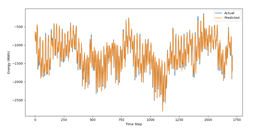
Figure 5: Predicted forecast compared to actual interconnection outflows from the testing data set. Remember, this portion of the dataset was completely unseen by the model.
My gut reaction: this is overfit. Honestly, I was not expecting to achieve such good results, but to explore if there was an obvious overfitting here, I created a Loss vs. Epoch chart for during-training validation, as seen in Figure 6.
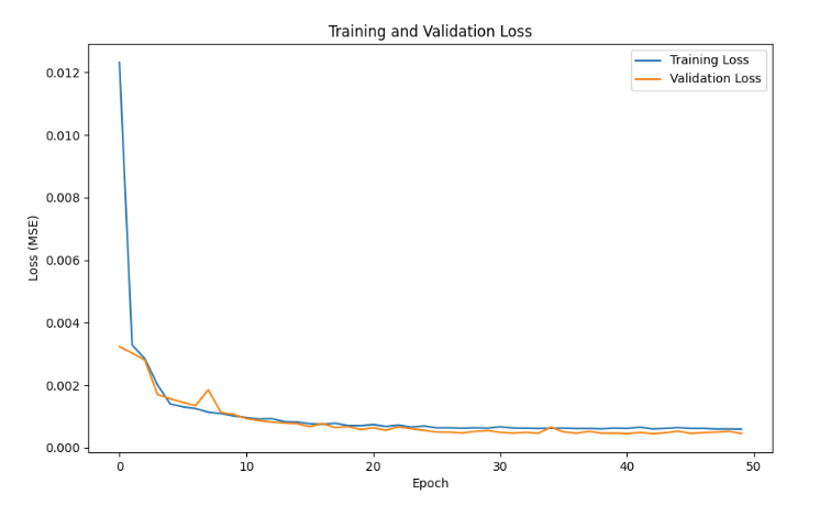
Figure 6: Training and Validation loss showing validation loss decreasing then holding constant as epoch numbers approach 50.
If the model was overfit, validation loss would increase as the number of epochs increased. In other words, an overfit model loses its generality with additional training and error increases as it can no longer accurately predict unseen data. Based on the validation loss not increasing at larger numbers of epochs, there are no indications of the model being overfit.
Conclusion: The Value of “Basic”
As AI races forward, it is worth remembering the foundations of machine learning can be immensely powerful tools, if trained, validated, and maintained properly. As exhibited in this article, two different models were applied to two different problems, each with promising results.
In my next blog post, I will continue validating this LSTM model and build on its application to the energy industry. Forecasting hourly interconnect flows is one thing, building actionable data insights is another.
References:
Berejnoi, A. (n.d.). How to implement backpropagation with NumPy. Medium. Retrieved from https://medium.com/@andresberejnoi/how-to-implement-backpropagation-with-numpy-andres-berejnoi-e7c14f2e683a
Deep Learning – Foundations and Concepts (Bishop, C. M., & Bishop, H.). (2023). Springer Cham. http://doi.org/10.1007/978‑3‑031‑45468‑4
GeeksforGeeks. (n.d.). tanh vs sigmoid vs ReLU. Retrieved from https://www.geeksforgeeks.org/deep-learning/tanh-vs-sigmoid-vs-relu/
U.S. Energy Information Administration (EIA). (n.d.). Electric power operational data [Dataset]. Retrieved from https://www.eia.gov/opendata/index.php/browser/browser/electricity/electric-power-operational-data
Why are RNN/LSTM preferred in time‑series analysis and not other NN? (n.d.). DataScience.StackExchange. Retrieved from https://datascience.stackexchange.com/questions/23029/why-are-rnn-lstm-preferred-in-time-series-analysis-and-not-other-nn#:~:text=Every%20neural%20net%20gets%20better,networks%2C%20the%20training%20time%20etc.
Georgia Institute of Technology. (2025). CS7646: Machine Learning for Trading [Course].
Best Performing Hedge Funds in the Last 10 Years (2024). LevelFields. Retrieved from https://www.levelfields.ai/news/best-performing-hedge-funds-10-years
Loved the article? Hated it? Didn’t even read it?
We’d love to hear from you.